Atoms, the Redshift and the Zero Point Energy
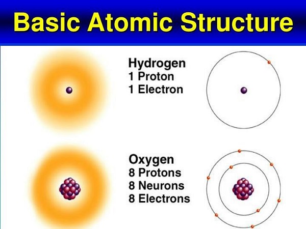
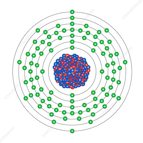
The number of sub-atomic particles making up an atom continue building for successively heavier elements. Each ‘shell,’ or level of electrons has an optimum number of electrons in it. As the elements build in atomic size, first the innermost shell of electrons is filled, then, one by one, the next shell is filled, and then the third shell becomes filled, and so on. The shells are successively filled as the number of electrons (and protons) associated with the various elements increases. The naturally occurring element with the most particles is Uranium. (Others may have more, but they have been artificially formed.) Uranium atoms have 92 protons and about 143 neutrons that make up the nucleus as shown in the image below. It also has 92 orbiting electrons in 7 levels or ‘shells’.
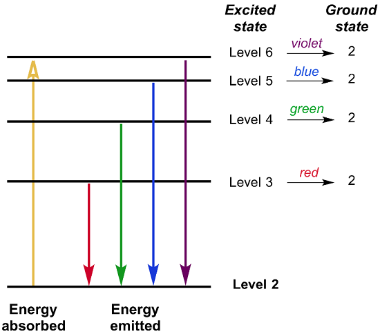
It is possible for something energetic, like a gamma ray, or some stray atomic particle, (E in the diagram below), to disturb an electron in its orbit. This disturbance can elevate an electron from its customary orbit to one farther out from the nucleus. The atom is then said to be “excited.” Such an atom is usually unstable and the electron will snap back to its customary orbit very quickly. When it does so, the energy which forced it into that outer orbit is released as a photon of light, as pictured below. This is explained more fully later, but all light photons have have an origin in the movement of electrons.
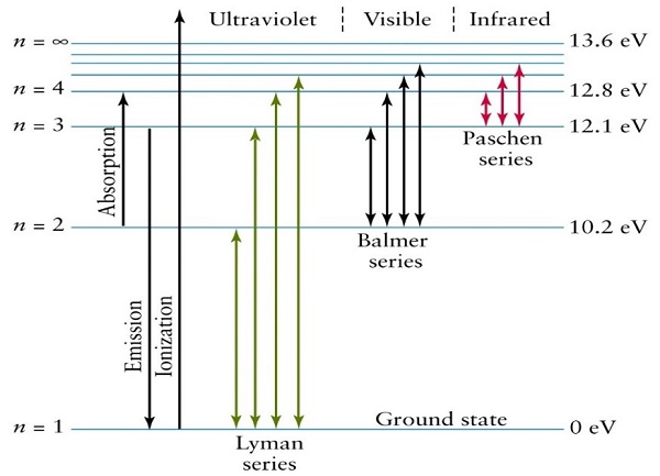
When such electrons transition back from an outer to an inner orbit, the color of the light photon that is emitted depends on the orbits involved. The closer the two orbits involved are, the redder is the light emitted. (The cause for this is discussed later, as it is not the cause which, up until now, has been commonly accepted.) The concept is illustrated below. There, the energetic source passing through the atom is given by the yellow line, with the upwards arrow, on the left, showing the energy absorbed as the electron is elevated to a higher orbit. On the right, 5 of the 7 electron shells or levels are shown. Then in the center of the diagram is a series of colored arrows dropping from an outer to an inner level, orbit or shell. In this, as an example, the transition from Level 3 to Level 2 is shown as emitting a photon of red light, while the fall from Level 6 back to Level 2 emits photons of violet light, and so on.
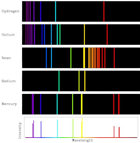
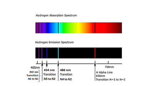
Because each of the 92 naturally occurring elements has a unique atomic structure, the light emitted by that atom is typical of the atoms of that element alone. The light emitted appears as bright lines and are called spectral lines. They are as characteristic as fingerprints or bar-codes. The instrument, which shows these lines clearly, is called a spectroscope. We can tell what element we are dealing with by these spectral lines. Here are some examples. From top to bottom we have Hydrogen, Helium, Neon, Sodium, & Mercury.
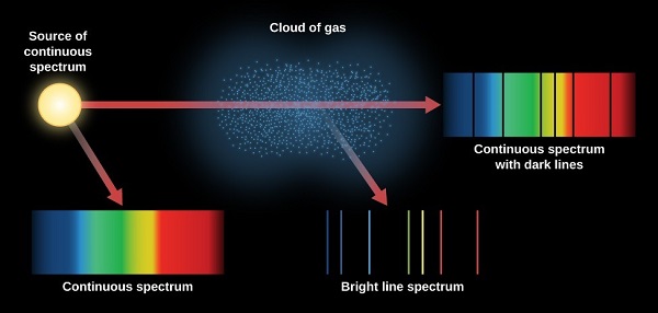
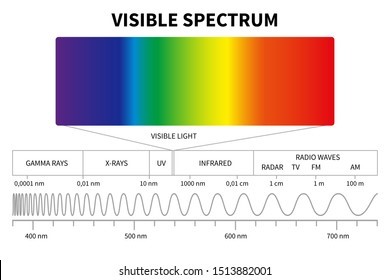
Because these emitted lines of specific colors are bright, they are called emission spectra. However, a source which has free electrons moving around, such as an incandescent lamp filament, or the surface of the sun or a star, can produce a continuous, or rainbow-like, spectrum instead of just discrete lines. This is shown in the image below on the bottom left panel.
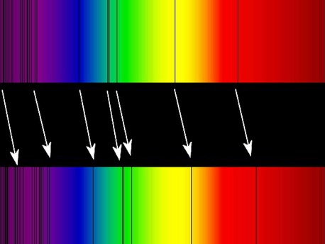
When light from the source of such a continuous spectrum shines through a cloud of gas, dark lines appear on the continuous spectrum as in the top right. These dark lines occur because that is where the gas atoms have absorbed their specific wavelengths of light. This is called the absorption spectrum. In space, some of these gas clouds are enormous – big enough to contain stars themselves. This means the gas cloud could be glowing with the energy from the star or stars. If the gas cloud were glowing, it would have a bright line spectrum on a dark background, as shown in the lower right hand part of the diagram above. Note that the bright lines exactly correspond with the positions of the dark lines, as a comparison between the bottom right and top right images shows above. Both the emission and the absorption spectrum tell us the element(s) making up the cloud. This is why, when we point a spectroscope to a star or a gas-cloud, we can see all the spectral lines. That tell us what elements are in the star or gas cloud. Similarly, when distant light shines through the atmosphere of a planet, the absorption lines tell us the composition of that planet’s atmosphere. Historical Background: Between 1912 and 1922, Vesto Slipher and Francis Pease, working at the Lowell Observatory in Arizona, took detailed spectral measurements of what they thought were simply spiral gas and star clouds. However, what they were looking at were 42 spiral galaxies. Something odd was noticed. On earth and in our solar system, all spectral lines were in their customary position on the color spectrum, exactly where the laboratory standard indicated they should be. However, the spectral line patterns of these spiral galaxies were nearly all shifted towards the red end of the rainbow spectrum. The sort of effect being noted is illustrated here:
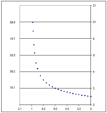
The spectral lines at the top come from the laboratory standard. The effect being observed with the spiral galaxies is seen at the bottom, where the same pattern of atomic spectral lines is systematically shifted towards the red end of the rainbow spectrum. During that same period, in 1923 and 1924, Edwin Hubble discovered Cepheid variable stars in the same spiral galaxies that Slipher and Pease had been working on. We have examples of these variable stars in our own neighborhood in space, so we know their behavioral characteristics. Cepheid variables are stars whose light output pulsates like clockwork. The bigger they are, the brighter they are, and the more slowly they pulsate. Their light curve revealed that the rise time to their peak brightness was always shorter than the time of decline to their minimum brightness. That is graphed here:
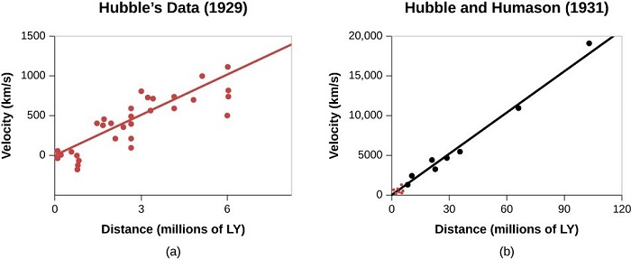
It had been found that such stars had an intrinsic brightness associated with their pulsation rate. In other words, knowing their pulsation rate from observation, we can know exactly how bright they are at a set distance. Then, when we measure how bright they appear to be, we then use standard physics to calculate how far away they are for their light to appear that dim. When Hubble did that for the Cepheids in the spiral galaxies, he received a surprise. Until that time, these “spiral nebulae,” as they were called then, were thought to be part of one entire and extensive Milky Way system. These distance measurements revealed that these “spiral nebulae” were so far away that they were quite separate from the Milky Way system altogether and were, in fact, their own “island universes” as these galaxies came to be known. They then began to understand that the Milky Way system was simply another one of these “island universes.” Pease and Pearson had measured the spectroscopic data. Hubble had examined the Cepheid variables in these same 42 spiral galaxies. Something unexpected emerged. Hubble discovered that the greater the distance of the galaxies, the larger the redshift. In 1929 he published his “Law of Spectral Displacements” which is now called Hubble’s Law. In its simplest form it states that the redshift of a galaxy is proportional to its distance from the point of observation. His 1929 graph is reproduced at bottom left. It shows data out to about 6 million light years’ distance. By 1931 Edwin Hubble and Milton Humason had cooperated to extend the spectral observations out to 100 million light years, and the Law was holding (bottom right graph) . Since then, the basic law has been verified to the limits of the cosmos. However, there has been much argument about the exact size of the proportionality factor between distance and redshift. This factor has undergone numerous changes since Hubble’s time up to the present.
The Doppler Interpretation: Essentially, though, Hubble’s Law is simply a redshift/distance relationship. As such it only notes that the redshift of light from galaxies is proportional to the distance of the galaxy. That is the basic data that astronomers and cosmologists deal with. If distance is R and the redshift is designated as z, then z is proportional to R and vice versa. The redshift, z, is a dimensionless number (a number on its own, without any units such as weights or distances connected to it). It is here that the trouble began. Although cautious about the procedure until more data came in, Hubble suggested that z be multiplied by the speed of light, c. This made R proportional to cz. This transformed a dimensionless number, z, into a velocity, cz. Hubble pointed out that this procedure allowed the redshift to be interpreted as a Doppler effect, with galaxies receding at a velocity, v, where v = cz. Hubble’s Law then became R = v/H, where H is the constant of proportionality called the Hubble constant. In order to understand what the Doppler shift means, it is important to understand that both light and sound have a full spectrum of wavelengths.
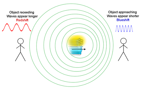
With light, the wave lengths are very short and energetic at the blue end and then become longer and less energetic at the red end. With sound, the higher sounds are the shorter and more energetic wavelengths and the lower sounds are the longer and less energetic wavelengths. In the mid-19th century Christian Doppler pointed out that the frequency of both light and sound waves changed with movement. The Doppler effect is shown in the diagram below. Basically, if an emitter of sound or light waves is moving, then the wave fronts crowd together (or are shorter) in front of the emitter, and trail out or lengthen behind it. This means that, for a stationary observer, the frequency or pitch of sound (or light) waves as the emitter approaches starts off high. It then drops as the moving emitter passes. As the emitter moves away, the pitch of the note gets lower, or, in the case of light, the waves look redder or more stretched out (longer).
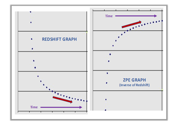
An everyday example is of a police car that passes you with its siren going. As it pulls away from you, the pitch of the siren drops. That is because the sound waves lengthen as the car passes you and moves away. In a similar way, Hubble suggested that the redshift, which shows lengthened wavelengths of light, might indicate that distant galaxies are racing away from us. Initial Problems with the Doppler interpretation: However, after 1960, a departure from linearity began to be noted as galaxy velocities appeared to begin to approach the speed of light. Consequently, by the mid 1960’s a relativistic form of the Doppler equation was introduced. Later, with the advent of the Hubble Space Telescope, that relativistic formula was found to be a reasonably accurate approximation for objects, even at the most distant locations. The graph below shows that specific redshift behavior coming forward from the beginnings of the universe on the left (the most distant objects), until now on the right (the closest objects). Note that the segment of the curve at the bottom right is approximately linear, in accord with the early values of z from galaxies closer to us seen in the graphs from Hubble and Humason in 1929 and 1931. In those two graphs, our galaxy is placed at the bottom left. In the graph below, our galaxy is at the bottom right.
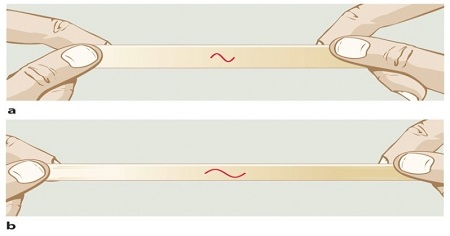
Doppler Redshifts and Einstein: Because of Hubble’s multiplication of the redshift, z, by the speed of light, c, a Doppler shift interpretation was given to the redshift data. This interpretation has led to the impression that galaxies are racing away from each other at speeds which increase with distance from our galaxy. Indeed, near the frontiers of the cosmos, those speeds are thought to be close to the current speed of light. Hubble himself had doubts about that explanation. Nevertheless, that was the explanation which was officially adopted. Even today, the Doppler Shift is the commonly accepted explanation for the redshift, and is taught in educational institutions. What aided the acceptance of the Doppler shift idea was the fact that Einstein’s field equations allowed an interpretation that the very fabric of space-time was static with the galaxies actually moving through it. This implied that the redshift was entirely due to galaxy motion, and so must be a Doppler effect. For many, this backing from Einstein’s equations ended all discussion. Other Scientists’ Reactions: Since the 1960’s, a number of scientists have questioned this approach. Is the redshift actually indicative of motion? In The Deep Universe, with B. Binggeli & R. Buser (eds.), p. 369 (Springer, Berlin, 1995), Malcolm Longair wrote: “Thus, redshift does not really have anything to do with velocities at all in cosmology. The redshift is a … dimensionless number which … tells us the relative distance between galaxies when the light was emitted compared with that distance now. It is a great pity that Hubble multiplied z by c. I hope we will eventually get rid of the c.” Another approach considers data from quasars of high redshifts greater than z = 1. For example, Misner, Thorne and Wheeler in their tome on Gravitation, p.767, (W.H. Freeman & Co, USA 1997), rejected the Doppler explanation on the following grounds. Using an argument similar to several other scientists, they state: “Nor are the quasar redshifts likely to be Doppler; how could so massive an object be accelerated to a speed close to light, without complete disruption?” In thus rejecting the quasar redshifts as Doppler effects, they also point out the problem that exists with one alternative explanation, namely gravitational redshifts. They state: “Observed quasar redshifts ranging from z = 1 to z = 3 cannot be gravitational in origin; objects with gravitational redshifts larger than about z = 0.5 are unstable against collapse.” So, in eliminating Doppler shifts and gravitation as the origin of the observed redshifts, they come to what they see as the only other solution, namely “a cosmological redshift.” The Alternative to Doppler– a Cosmological Redshift: As early as the late 1920’s, in a modification of Einstein’s work, Friedmann and Lemaitre produced equations showing that space itself might be expanding, whereas Einstein considered space to be a fabric which was fixed. Friedmann and Lemaitre’s theory was that, as the fabric of the universe expanded, then photons of light traveling through space would have had their wavelengths lengthened, causing a redshift. This was a cosmological cause for the redshift as the behavior of the fabric of space was in view here and that lengthened waves. The concept is illustrated here:
In these diagrams, a wave is drawn on a piece of unstretched elastic fabric. Then the fabric is stretched. As it does so, the wavelength is stretched proportionally, as in the bottom diagram. This is how they proposed that expanding the fabric of space lengthens wavelengths producing a redshift of light waves in transit through space from distant galaxies Actual data tend to negate this suggested cause as well. These arguments are discussed in detail in “Cosmology and the Zero Point Energy,” Chapter 5 (B.. Setterfield, NPA Monograph 2013, No. 1). But the important one here is a conceptually simple idea. If light-waves are being stretched as they go through the fabric of space, there should be significant broadening of the narrow spectral lines as well. Some broadening does occur in a few cases, but they are usually related to strong magnetic fields or other known effects. The rest of the lines are narrow and sharp. The preponderance of sharply defined, narrow spectral lines is a strong indication that the redshift is not from a continuing expansion of the fabric of space. Two important questions:
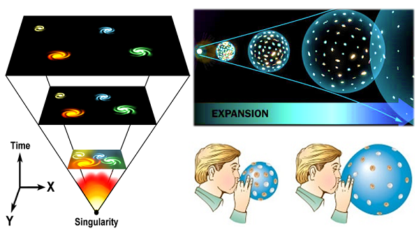
Some deny that expansion has occurred and consider the cosmos to be an entirely static entity. Again, that is not what the data indicate. The data strongly indicate that there was an initial, rapid expansion. Among those who accept universal expansion, it is usually assumed that the initial expansion of the universe is ongoing. However, there are scientists who point to data which deny any current expansion. Hydrogen cloud data provides a good example. In an early, smaller universe, objects were much closer together. As expansion continued, the distance between hydrogen clouds and all objects increased, as in the sketched examples below.
Hydrogen clouds have a special signature in their light spectra, which allows us to determine their distance and spacing. This has allowed us to determine the fact of the initial expansion of space (see for example Lyndon Ashmore, Proceedings, 2nd Crisis in Cosmology Conference, ASP Conference Series Vol. 413, 2008,. F. Potter Ed). At first, these hydrogen clouds were crowded together; then, as the cosmos expanded, they became farther and farther apart. This continued to a redshift (z) distance of z = 2.6 when slowing of the separation rate was noted. Coming closer to Earth, and thus forward in time, at a distance of z = 1.6, the clouds stopped separating altogether. They have stayed roughly the same distance apart ever since. The indication is that cosmic expansion stopped around a time corresponding to a distance of z = 1.6. If cosmic expansion stopped at z = 1.6, that means that from our point in space and time to that point in space and time, there has been no change in distance between the hydrogen clouds. It is before that point in space and time (which means farther out) that we see the changes in distances between the clouds. That means that the expansion was earlier in time but not continuing. This leads to the inevitable conclusion that the redshift we see in distant galaxies cannot be attributed directly to universal expansion. All of which creates another problem: If expansion has stopped, that means the universe today is essentially static. This raises the issue of the stability of a static universe. If the universe is truly static, then it should collapse under its own gravity. In 1993, in the Astrophysical Journal, 405:1, (March 1st), pp. 51-56, astronomers Narlikar and Arp published an analysis which showed that a static universe with matter in it would be stable against gravitational collapse, providing there was an oscillation involved. Similar scenarios had also been offered earlier by V.S. Troitskii (Astrophysics & Space Science, 139 (1987), pp. 389 ff). and T.C. Van Flandern (Precision Measurements and Fundamental Constants II, pp. 625-627, B.N. Taylor & W.D Phillips -Eds., NBS US Special Publication 617, 1984). They had proposed that, in order to maintain the stability of the universe as a whole, variation in some associated atomic constants was necessary, along with an oscillation. These suggestions indicate that the redshift need not be related to motion. (It needs to be understood that a slightly oscillating universe is still considered a ‘static’ universe as opposed to a current universe which is considered to be rapidly expanding.) If our universe is now static, with only slight oscillations, then the standard explanation for the redshift, which depends on an expanding universe, is called into question. The quantized redshift: The idea that the redshift is not related to movement or velocity received confirmation from a different, and controversial, set of data. William Tifft was the astronomer at the Steward Observatory in Arizona. From 1976, when he wrote the first of a number of papers, right up until 2014, when he wrote the book “Redshift – Key to Cosmology,” he called attention to a discrepancy in redshift data. He pointed out that, instead of smoothly increasing as we go away from our Local Group of galaxies, the redshifts appeared to be clumped or grouped or, more specifically, appeared to change in jumps. This came to be called the quantized redshift. If the redshift was actually due to galaxies racing away from each other as the Doppler explanation requires, then these speeds of recession should be smoothly distributed like cars accelerating down a highway. That is, the redshift should be a smooth curve. But the results Tifft was finding indicated that the redshift measurements jump from one plateau to another, like a set of steps. It was as if every car on the highway traveled only at speeds that were multiples of, say, 5 miles per hour, with nothing in between. It was difficult on either the Doppler model or the Lemaitre model to see how any cosmological expression of space-time expansion, or, alternately, the recession of galaxies, could go in jumps. Even more puzzling was the fact that some jumps actually occurred within galaxies. If the redshift was due to motion, then a change in redshift within a galaxy would mean that different halves of the galaxy were moving at different speeds. That would force the galaxy to disrupt; but it obviously was not occurring. So, redshift quantization tended to discount both the Doppler and Lemaitre models for universal expansion. One additional fact was especially puzzling; over a period of time, measured values of the redshift of some galaxies actually showed a reduction in their redshift, not an increase. This result did not fit the ideas of an expanding universe in any form.
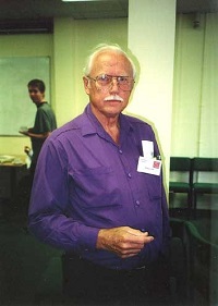
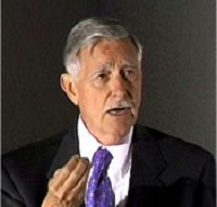
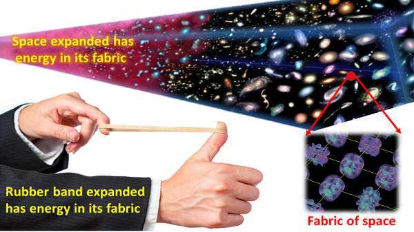
Tifft (above left) was not alone in his discoveries. He was supported by Halton Arp (center), Fred Hoyle, Geoffrey Burbidge and other great astronomers who added to the examples being collected. This did not go unchallenged. In an attempt to prove Tifft and the quantization of the redshift wrong, William Napier (above right) and Bruce Guthrie of the Royal Observatory, Edinburgh, used the most accurate hydrogen line redshift data available as well as doing their own measurements. By early 1991, they had developed and applied very rigorous statistical tests to galaxies in the direction of the Virgo cluster. By the end of 1991, they had studied 106 spiral galaxies detecting a quantization of about 37.5 km/s, close to Tifft’s quantum multiple of 36.2 By November of 1992, a further 89 spiral galaxies had been examined and a quantization of 37.2 km/s had emerged. In 1995, they submitted a paper to Astronomy and Astrophysics with the results from a further 97 spiral galaxies showing a 37.5 km/s quantization. One argument the critics used was that the quantization only appeared because the sample sizes were so small – not enough galaxies had been studied. So they were asked to repeat their analysis with another set of galaxies. In 1996, 117 additional galaxies were used. The same 37.5 km/s quantization was plainly in evidence. That same year, Astronomy & Astrophysics accepted B.N.G. Guthrie and W N. Napier’s paper [vol. 310, pps. 353 ff.]. The possible error in measurement was only 1/10th the size of the quantization. A Fourier analysis of all 409 data points showed a huge spike at 37.5 km/s with a significance of one in a million. This means there is only one in a million chance of this result being mere coincidence. Other astronomers persisted with these studies. For example, in 2010, Halton Arp and his colleagues noted that if quasar clusters are examined, and the central redshift is taken, then the redshift differences hover around the redshift values of z = 0.06; 0.30; 0.60; 0.96; 1.41; 1.96 and 2.64 with most at z = 1.96. It has become standard to try and explain away many of these results by the action of “dark matter.” We must point out that, despite extensive searches, dark matter has never been found. (It is mathematically necessary for some models, but has never been actually found.) If the Lemaitre model is true, space must be expanding in jumps. On the Einstein-Doppler model, the velocity of recession of galaxies must vary in jumps, or fixed steps. Because both these options are highly unlikely, we need to re-think our ideas and look at other options. Quantization does not answer the redshift problem, but it does show there is an additional factor to this problem which needs to be resolved. The New Tired Light Hypothesis: Apart from what will be presented here, there is only one other proposed model that has been presented to explain the redshift: the New Tired Light Model. This model was designed to accompany the idea of an entirely static universe. In that model it is proposed that “photons of light from distant galaxies are absorbed and re-emitted by electrons in the plasma of intergalactic space, and on each interaction the electron recoils. Energy is lost to the recoiling electron (New Tired Light Theory), and thus the re-emitted photon has less energy, a reduced frequency and therefore an increased wavelength. It has been redshifted” [Proceedings NPA 17th Conf. Long Beach, CA, 2010, pp.17-22; Proceedings NPA 19th Conf. Albuquerque, NM, 2012, pp.17-19, etc]. This model is still being pursued by some. However, it has difficulty in accounting for redshift differences or quantizations between pairs of more or less equally distant galaxies. Secondly, it is awkward to explain on this model how a redshift change can go through a single galaxy. Finally, it also fails to account for the observational data that some redshifts have dropped by one quantum change over time. A suggestion that also answers one problem: With data itself mitigating against galactic motion, space expansion, and the New Tired Light model, there seems to be only one option left. This is the one first mentioned by John Gribbin on 20th June, 1985 in New Scientist on page 20. He hinted that the redshift may be due to something happening with the atomic emitters of light themselves. If this is indeed the case, there is no need to consider a change in the wavelength of light in transit; the wavelength would be fixed at the moment of emission. This also avoids a difficulty that Hubble perceived in 1936, namely that “…redshifts, by increasing wavelengths, must reduce energy in quanta. Any plausible interpretation of redshifts must account for the loss of energy.” [The Realm of the Nebulae, p.121, Yale University Press, 1936]. In other words, if the high energy original light photons somehow were shifting to the lower energy, redder, wavelengths, where did the extra energy go? There is a basic law in physics that energy is conserved. The conservation of energy from light photons (quanta) in transit has always been a problem for cosmologists. Some have actually claimed that this is one case where energy is not conserved [E.R. Harrison, Cosmology, The Science of the Universe, p.275-276, Cambridge University Press, 1981]. If, however, the atomic emitters themselves are responsible for any changes we observe, this alters the problem entirely. If the wavelength of the light, whether it is different from our earth standard or not, is established at the moment of emission, then energy conservation in transit is no longer an issue. Since the amount of red-shifting is also considered an indicator of distance, the cause of the redshift must be universal. With everything else eliminated, except the behavior of the atoms themselves, this means that whatever is affecting atomic emitters must also be universal. Earlier, we noted that atoms are made up of charged particles. As a result, they are electric and magnetic in character, and in their behavior. Consequently, their behavior depends on the electric and magnetic properties of the vacuum of space. The physical quantity which controls those properties in the vacuum of space is called the Zero Point Energy or ZPE. The ZPE: Most scientists agree that the universe expanded at the beginning. (Although this was originally given the derogatory name of “Big Bang” by those supporting a static universe, there was no ‘bang’ involved, but rather a very rapid expansion.) As the fabric of space was stretched out, the galaxies became farther apart. Stretching the heavens was like inflating a balloon. As the stretching goes on, the potential energy in the fabric of the balloon builds up. An expanded rubber band also has potential energy. In both these examples, the potential energy is released as kinetic energy when the balloon or rubber band is let go. Likewise, as space expanded, the potential energy was converted to the kinetic energy that we now recognize as the Zero Point Energy. This energy, existing in all waves of the electromagnetic spectrum is pervasive throughout the universe.
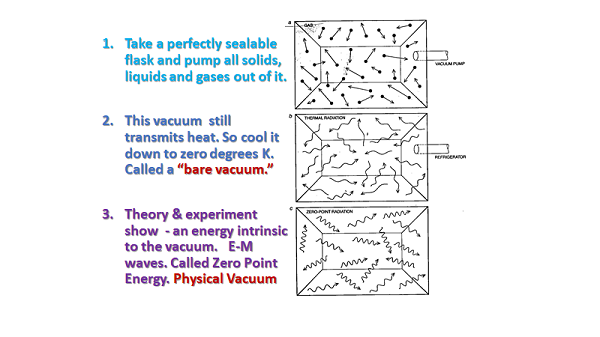
How was the ZPE discovered? Wrong! In the 19th century, it was found that there was still temperature radiation in this vacuum. So the flask was cooled to close to zero degrees Kelvin – which is absolute zero (minus 460 degrees F, or minus 273 degrees C). This was referred to a ‘bare vacuum.’ That was not the end of it. In the early 20th century it was discovered that there was an energy there, intrinsic to the vacuum. Because that energy exists even at absolute zero temperature in an actual vacuum, it has been called the Zero Point Energy. The real vacuum in which this exists is called the Physical Vacuum. This sequence is illustrated here:
We are not aware of the presence of the all-pervasive Zero Point Energy (ZPE) for same reason we are not aware of the 14 pounds per square inch of atmospheric pressure on our bodies. It is the same inside and out. The ZPE exists inside all our measuring devices and all matter as well throughout the universe. One way in which the ZPE was confirmed was through something called the Casimir Effect. Other confirmations followed:
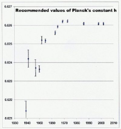
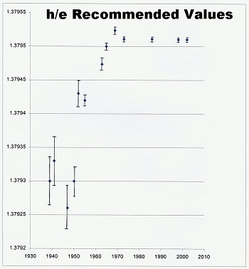
ZPE characteristics: The ZPE exists as random (or stochastic) interacting waves. Experiments show the ZPE is comprised of electro-magnetic waves of all wavelengths. It has a preponderance very short wavelengths as opposed to long ones. In fact, the multitude of short waves is great enough so that atoms and subatomic particles are jiggled around at the incredible rate of over 1020 (that is 100,000,000,000,000,000,000) hits per second. On the other hand, there are so few waves the size of objects we can see that none of it jiggles. The study of these random ZPE waves and their effects is part of the field of Stochastic Electro-Dynamics, or SED physics. There is a two-fold aspect to these ZPE waves. This picture may explain it: When cross-current ocean waves meet, they crest and peak and form whitecaps. Whitecaps don’t last, but soon disappear. Similarly, when energy waves of the ZPE meet, the concentration of energy becomes something referred to as a virtual particle pair. In this pair, one is positively charged and the other is negatively charged. They are referred to as “particles” because for the instant of their existence, they behave as particles. Then, because positive and negative attract each other, they slam back together, annihilate, and return to ZPE energy. This happens because energy and matter are inter-convertible. So, the ZPE can be viewed from either a wave or a particle approach.There are a multitude of different types of virtual particle pairs, including, but certainly not limited to protons and anti-protons, electrons and positrons, positive and negative pions, etc. At any instant today, there are about 1058 virtual particle pairs per cubic inch. The positive and negative charges of the virtual particle pairs, along with the Zero Point Energy itself, control the electric and magnetic properties of the vacuum of space. At the beginning, as cosmic expansion continued, the potential energy of the expansion continued to convert to the kinetic energy of the ZPE. Space then got “thicker” with energy and virtual particles. In other words, an increase in ZPE strength, due to universal expansion, changed the electric and magnetic properties of the vacuum of space. The Zero Point Energy affects all atoms and atomic emitters. It maintains electrons in their orbits around the nucleus. These orbits have two conditions that must be met simultaneously; first a constant energy (potential and kinetic combined) in the electrostatic field of the nucleus; second, a momentum as described by Planck’s constant. SED physics points out that Planck’s constant, h, is proportional to the strength of the ZPE. Since the ZPE originated with the expansion of the cosmos, and its strength smoothly built up with time as the cosmos expanded, h also smoothly increased. Some of that increase in Planck’s constant, h, can be seen on these graphs of recommended values of h as well as h/e (Planck’s Constant over the electronic charge) from the Bureau of Standards since measurements first began.
The lower strength of the ZPE in the early cosmos resulted in a lower momentum of electrons in their orbits. This, in turn, meant that the light they emitted was redder then. It became bluer with time as the ZPE strength built up. This explains the increasing redshift as we look back to progressively more distant, and hence older, objects. There is also a possible suggestion using this ZPE approach as to how the 37.5 km/s quantization might have originated. This is discussed in more detail below.
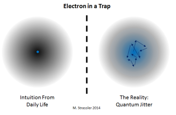
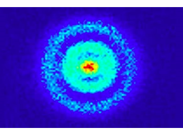
Here are three pictures of the behavior of electrons. The one on the left was what was expected historically. However, the one in the middle is what we found actually occurred. Because of the extremely high numbers of very short wavelength ZPE waves, all atomic particles undergo intense battering by the ZPE. Electrons are hit by the impacting ZPE waves causing them to jitter back and forth 1.23 x 10²⁰ times per second. This rate is called the Compton frequency, C*. For this reason, electron orbits, as shown on the right, are fuzzy. The right hand image is a photo of a hydrogen atom with an electron going around in its orbital showing effects of ZPE impacts causing a Jitter. An electron is hit about 18,770 times each orbit. (This is determined by dividing the Compton frequency, C*, by the frequency or number of times per second the electron goes around in the 1st Bohr orbit. That quantity is listed as 6.579 x 10¹⁵ per second. The result of the calculation reveals that there are about 18,770 hits per orbit) This gives the orbit the fuzzy outline seen on the far right. The ZPE and atomic orbits: In order to understand the next part, two definitions have to be made clear: velocity and acceleration. While we refer to a car speeding up as accelerating, that is not what acceleration means in physics. In classical physics, the term ‘velocity’ refers to a speed in a certain, given direction. A change in that direction means a change in velocity which, in turn, is then defined as acceleration. If either speed or direction changes, it is defined as an acceleration. And one of the consequences of acceleration is the radiation of some amount of energy. When an electrically charged object, like an electron, changes direction (as it must in its orbit), it is undergoing acceleration and hence is radiating energy. Since that electron is continually changing direction, it is losing energy and hence should spiral into the nucleus and the whole structure should disappear in a flash of light. That does not happen, but why not? Classical physics had no real answer to the energy loss. Quantum physicists set the phenomenon as a Law that says an electron does not radiate energy when moving in a stable orbit. Why this was made a quantum Law is not discussed. Rather, quantum physicists talk about the wave patterns of the electron reinforcing. But that is no answer if energy is being lost. Why? Because those reinforcing wave patterns will gradually lose more and more amplitude, (the distance between the peaks and troughs of the waves, that is the height of the waves), until there is no wave pattern left at all. At that stage, the structure would cease to exist. SED physicists point out that classical physics is correct when it states that orbiting electrons radiate energy. However, the factor which has been ignored by both classical physicists and quantum physicists is the contribution of the Zero Point Energy. The energy that electrons radiate as they orbit their protons can be calculated, along with the energy they absorb from the ZPE. As SED investigation proceeded, it was found that for a stable orbit, the energy lost by the orbiting electron was equal to the energy imparted by the ZPE impacts. It was found that the equilibrium (stable) orbit radius for a hydrogen atom was equal to the 1st Bohr radius if circular orbits were considered. Indeed, “for smaller distances, the electron absorbs too much energy from the ZPE field…and tends to escape, whereas for larger distances, it radiates too much and tends to fall towards the nucleus.” [de la Pena in ”Stochastic Processes applied to Physics and Other Related Fields” pp. 428-581, B. Gomez et al., Eds, World Scientific Pub. Co., 1983].
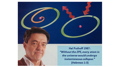
In 1987, Hal Puthoff wrote a key paper on this topic in Physical Review D for May 15th. He concluded with the comment that this whole idea “carries with it the attendant implication that the stability of matter itself is largely mediated by the ZPF phenomena in the manner described here.” In another forum, he stated that “Without the ZPE, every atom in the universe would undergo instantaneous collapse.” How does it work? The scenario which emerges was outlined by Spicka et al. in the Spring Conference, “Beyond the Quantum,” 2006, The Netherlands, which discussed the role of SED physics in explaining quantum phenomena. They pointed out that an electron moving in an orbit around a proton is under the influence of its electrostatic attraction. It is in terms of this electrostatic field of the nucleus that the electron’s potential and kinetic energy are measured. As it moves, the electron undergoes a series of elastic collisions with the impacting waves or photons of the ZPE which perturb this orbit around the nucleus. These impacting waves or photons force the electron to change direction. When this happens, the electron emits recoil radiation, just as classical physics explains. The electron’s whole ‘orbit’ then becomes composed of a series of essentially straight line segments whose direction is continually being changed by the momentum imparted to the electron by the impact of the ZPE waves or photons.
This example shows that the initial momentum of the system equals the final momentum. One ball of mass, m, coming in with velocity, v. is equal to one ball of the same mass, m, finally going out, with the same velocity, v. The momentum is defined by the product, mv. In a similar way, the kinetic energy coming in also equals the kinetic energy going out, where kinetic energy is defined as ½ mv2. In an inelastic collision, using, perhaps, marshmallows instead of iron balls, the marshmallows would absorb the vast majority of the energy, so the kinetic energy in would not equal the energy out. A perfectly inelastic collision would result in a final velocity of zero. Consider what happened to mass and velocity as the stretching of the cosmos continued. The result of the stretching was that the strength of the Zero Point Energy (ZPE) smoothly increased as outlined above. In terms of an electron, it would be hit and jiggled by an increasing number of waves or photons per second. Thus, the number of impacts per unit area per unit time on the electron would increase. The velocity of an electron is, in part, dictated by the number of ZPE waves it is battered by. As the ZPE strength increases, the number of waves per given volume also increases. The result is that the ZPE is effectively offering greater resistance to the motion of the electron in its direction of travel. This impedes the motion of the electron and thereby lowers its velocity. So, as the ZPE strength increases, electrons are forced to travel more slowly in their orbits. This gives us an inverse relationship between ZPE strength and electron velocity. Because this relationship applies generally, it is also true for the motion of particles in the nucleus itself, as well as for electrons orbiting outside. The mathematical analysis for this is in the NPA Monograph No. 1 for 2013, “Cosmology and the Zero Point Energy,” which indicates that sub-atomic particle velocities, v, can be shown to be inversely proportional to the ZPE strength, U. That is to say, as the ZPE strength, U, increases, the particle velocity, v, decreases. So mathematically, v is proportional to 1/U, or, alternately, 1/v is proportional to U. It is also important to understand that the impacting waves of the ZPE “jiggle” all atomic particles at speeds close to the speed of light. This is because, as SED physics has shown, subatomic particles are essentially charges. This means their intrinsic mass is close to, if not actually, zero. Einstein, however, showed that mass and energy are interconvertible. As a result, this jiggle imparts an energy of motion to the particle which, from modern physics, has a mass-equivalence. It is this mass which the subatomic particles possess, and it comes from the ZPE jiggling. Haisch, Rueda and Puthoff have discussed this fully and quantified it mathematically in Physical Review A, 49, pp.678-694 (1994); The Sciences, Nov./Dec. 1994, pp.26-31, and elsewhere. The formula that emerges from the mathematical treatment of this phenomenon shows that the atomic mass, m, is proportional to the square of the ZPE strength. That is to say, mathematically, m (subatomic mass) is proportional to U2. Two different results: It can also be shown that particle potential energies in the field of the positively charged protons in the atomic nucleus will also remain constant. Thus, for any orbit of given radius, r, the sum of the potential and kinetic energies will remain unchanged regardless of ZPE strength. In other words, the ZPE can vary but the sum of potential and kinetic energies remains constant. This satisfies the first of two equations governing the behavior of orbiting electrons. The situation for momentum is different. Momentum is given by mv, where mass, m, is again proportional to U2, and velocity, v, is proportional to 1/U. Thus momentum, mv, is proportional to U2 multiplied by 1/U which is proportional to the ZPE strength, U. The same holds true for the moment of momentum or angular momentum which incorporates the radius, r, of the orbit in its formulation as mvr. This means that, as the ZPE strength increases, it causes an increase in the mass of the electron. This means that the orbital momentum of the electron also increases in proportion for any orbit of a given radius, r. This information about the orbital momentum of an electron leads into the conclusion reached by Puthoff in his 1987 article. There, he demonstrated that the ZPE supported all atomic orbital structures by feeding into the angular momentum of the electron, providing it with the energy needed. This is in accord with the second of the two equations governing the behavior of orbiting electrons where mvr is equal to a multiple of Planck’s constant, h. Because SED physics shows that h is a measure of the strength of the ZPE, as the ZPE smoothly built up with the stretching of space, Planck’s constant similarly increased. The orbital angular momentum of the electron then also built up smoothly, as the equation demonstrates. A little more technical explanation Atomic orbital transitions
The outcome of these considerations is the standard diagram shown here. The atomic orbits are shown for which the moment of momentum has the letter n equal to n = 1; n = 2; n = 3; n = 4; etc. Here it is understood that this means n times h/(2π), so these values of n are, in reality, multiples of h/(2π). Remember that the actual value of h, and/or the moment of momentum, depends on the ZPE strength. Each of these stable orbits with a fixed n value has a total energy (in the electrostatic field of the nucleus) that is made up of the kinetic plus the potential energy associated with that orbit. As we saw above, this orbit energy is fixed for all values of ZPE strength, and is given in electron Volts, eV, on this diagram. It is the orbital moment of momentum, or angular momentum, not the total energy, that varies with h. It has already been stated here that a photon of light is emitted when an electron, forced farther out from its original orbit (or place), snaps back to where it belongs. The diagram above also shows the three series of spectral lines for hydrogen associated with an electron snapping back from an outer orbital to an inner orbital with a lower value of n and hence a lower quantum value of h. Looked at in this way, these spectral lines are actually the result of different values of h for different orbitals with their different moments of momenta. This fits in well with the changing values of h as the universe expanded and the ZPE built up. Thus the orbit potential and kinetic energies are fixed for all ZPE strengths (as measured by h, or Planck’s Constant). This means that the orbital radii, r, and the specific value of n for each orbital are also fixed. If h at a later time was twice the size of h earlier, then the quantity nh/(2π) would have twice the size for all values of n. Since this would indicate a more energetic version of h, then all emitted light photons from these atomic orbital transitions would be more energetic or bluer at this later time. Since h is measured in Joule-seconds (Joules multiplied by seconds) and Joules are the measure of energy, then a higher value for h means more Joules are associated with this value since the measure of time, the seconds, has remained the same. This then means that the higher energy difference in h between fixed orbitals, will result in bluer, or more energetic, light being emitted. What is being proposed: Mathematically
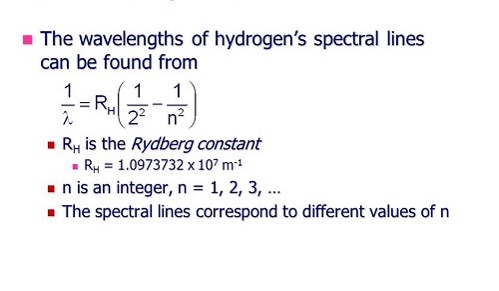
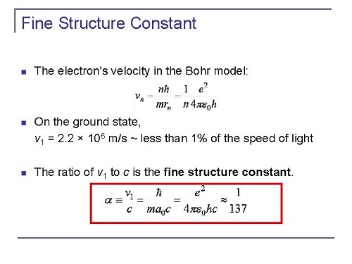
In 1890, Rydberg noticed that the inverse of the wave-length, that is, 1/λ, of the respective lines form a sequence given by A possible cause for the redshift: This leads us to the following conclusions. If the spectral lines are coming just from the orbit energy, their wavelengths, λ, will obey relationship (1) given by 1/λ = R( [1/n02 ] – [1/n2 ] ) (1) Alternately, if the spectral lines are the result of the change in momentum and Planck’s constant h rather than energy, then wavelengths, λ, will obey relationship (2) given by 1/λ = HR( [1/n02 ] – [1/n2 ] ) (2) Note that in relationship (2), the quantity H is simply the ratio of Planck’s constant at the time of emission, he, compared with Planck’s constant now, h. Thus, at any given instant when the ZPE strength has not changed, H = he /h = 1. This is the current situation on earth now. Consequently, relationship (1) and relationship (2) have the same result. It is only as we look out into space where we are effectively looking back in time, that the light emitted by atoms occurred when the ZPE was lower, and so he was lower than h. In that case, H was different from now. If, for example, the ZPE strength was only 0.5 or half of what it is today, thenhe is 0.5 of what h is today. Therefore H = 0.5. In relationship (2), this means that the inverse of the wavelength of light emitted, that is 1/λ, is equal to 0.5, which means that the wavelength, λ, is twice as long as currently measured. Since longer wavelengths mean redder light, then a redshift of light will have been recorded from that distant object. Yet there is another factor in (2) which needs attention; let us introduce it this way. ZPE Effects on Atoms and the Fine Structure Constant, Alpha: We have already noted that the Compton frequency, C*, for the electron is, according to SED physics, the number of hits on the electron per second by the impacting waves or photons of the Zero Point Energy. We saw that C* was equal to 1.2355 x 10²⁰ hits per second, which meant that the electron was hit about 18,770 times each orbit since the electron completes 6.579 x 10¹⁵ orbits per second in the 1st Bohr orbital. This figure of 18,770 hits per orbit surprisingly leads us to another atomic quantity, the fine structure constant, α (Alpha). Alpha is a dimensionless quantity which has a value very close to 1/137. Sommerfeld, who originally introduced the fine structure constant in the early 20th century, pointed out that its numerical value was equal to the velocity of the electron in the 1st Bohr orbit divided by the speed of light. This relationship is still retained today as in this example: Thus, the velocity of the electron in its orbit is less than the speed of light by the factor of Alpha. The velocity of the electron is also moderated by its physical interaction with the ZPE by a consistent factor that is 137 times greater than the interaction of light photons with the ZPE. Thus, the electron speed is 137 times smaller than the speed of light. (This explains the proportionality factor is between the speed of electrons in their orbits compared with the vacuum speed of light.) It is this electron, whose properties are moderated by the ZPE, which is giving rise to the spectral lines and their effects. So there is a moderation factor involving Alpha when comparing any ZPE changes with its effects on the atom. This is confirmed by a different example. A detailed examination shows some apparently single spectral lines have actually been split to become very close double or multiple lines. This splitting apart of the original line is called ‘fine structure’ to the line. The explanation often given is that fine structure arises because the electron has an intrinsic angular momentum, which we have seen comes from the electron’s interaction with the ZPE. A charge in motion is the definition of an electric current in standard physics. Thus an electron in motion is an electric current. The orbiting electron has a magnetic field associated with it since electric currents always have a circling magnetic field. That magnetic field interacts with the electron’s angular momentum. As a result of this interaction, the fine structure constant, Alpha, reveals how the spacing between the lines has been suppressed or contracted. The relevant equation shows that this contraction is given by a factor of α2, or (1/137)2 or 1/18,770. In other words, for the splitting of single spectral lines, those lines are closer together by a factor of about 18,770 times more than might be expected from other considerations. (See: https://physicsworld.com/a/theory-experiment-and-fine-structure/ ) Thus there are links between the number of ZPE hits which impart angular momentum to the orbiting electron and the splitting apart of some spectral lines. This confirms that Alpha is linked with both the ZPE and atomic behavior and that atomic spectra are moderated by factors involving Alpha. Now let us turn to the basic question asked earlier. What is the proportionality factor between the difference in the measured length of the same spectral line back in the past and today’s length compared with the change in the strength of the ZPE on those two occasions? To answer that question, let us go back to equation (2) above. There we find that the effects of H on wavelength are moderated by a factor of R in such a way that 1/λ is made bigger by R. This means that, if 1/λ is bigger, then λ is made smaller by this factor R. This means that the differences in the measured length of the same spectral line will also be moderated by the factor R. The problem is that the Rydberg constant is in units of length while the proportionality factor must be dimensionless, that is, without units (without mass, or weight, or length, or time, etc.). In this regard, it has been noticed by several commentators that the Rydberg constant, R can be expressed to an accuracy of 0.1% as the ratio of α3 /4πre where Alpha is again the fine structure constant and the quantity re is the classical electron radius. [See for example: https://energywavetheory.com/physics-constants/rydberg-constant/ ] Let us designate 4πre as Re, the enhanced electron radius, which will be useful later. For now, we examine the moderating effects of Alpha. When this is done, equation (2) then indicates that both the wavelength and the differences in wavelength are made smaller by a factor of (137)3; that is 2.5713 million. Therefore, since the redshift or wavelength difference, z, approximates to 2000 when the Cosmic Microwave Background Radiation (CMBR) was formed near the origin of the universe, this means that the ZPE has increased since then by a factor of (2000) x (2.5713 x 106) which is equal to 5.142 x 10⁹. We have a cross-check on this from Compton frequency data which shows that the ZPE has increased by a factor of about 3.13 x 10⁹ since the formation of the CMBR. This was preseted at a virtual Conference, as well as near the end of a YouTube session here: https://www.youtube.com/watch?v=-J6rbzuhsKM
What is the cause of the Redshift Quantization? 1/λ = HR( [1/n02 ] – [1/n2 ] ) (2) There are only two quantities in (2) that are amenable for quantization, namely H and R. In a changing ZPE sitaution with ongoing cosmic expansion, H is simply a ratio of the value of Planck’s constant at the time of emission compared with h now. Since h is changing smoothly, this is not open to quantization. So we turn our attention to the composition of R, which is closely approximated to the ratio of α3 / Re , where Alpha is again the fine structure constant and the quantity Reis the enhanced electron radius introduced above. Since the redshift, z, is measured by wavelengths, then we need λ from (2) rather than 1/λ . This means the quantization will involve the quantities in the Ratio Re / α3. Let us pull out of Re one of its factors, namely 3πα/4. Then the quantity Alpha again assumes some importance. The Ratio Re/ α3 then becomes [3π/(4α2)][Y] where Y contains the dimensional component (that is the physical radius of the electron) while [3π/(4α2)] is the quantization factor which is being repeated. This can then be shown to be the repeating factor in redshift, z, which is also dimensionless, and numerically equal to 1.2553 x 10⁻⁴. When this factor of z is multiplied by the speed of light, c, or 299,792 km/s, the result is the observed quantization of 37.6 km/s. Finally, the dimensional component of the electron radius, Y, from the above figures is near 8.15 x 10⁻¹⁷ meters. This is in accord with the latest experimental evidence from scattering experiments, work from the LHC, and other lines of enquiry which all suggest that the physical dimension of the electron is around 10-18 meters. Thus Y turns out to be the radius of the electron. Concluding Summary: Barry Setterfield. 21st August, 2021.
|